The very first Machine Learning model when we start learning is Linear Regression.
The idea of Linear Regression is simple. We’re given a data with a set of features and output range is continuous. Our task is to find a best line (plane in 3D and hyperplane in multi-D) that has the error between the line and outputs is as close as possible.
The most popular loss for regression is Mean Squared Error (MSE) which has the form:
\[J(\mathbf{w}) = \frac{1}{2M}\|\mathbf{h(w)} - \mathbf{y} \|_2^2\]Suppose we have a matrix dataset: $\mathbf{X} = (\mathbf{x_1}, \mathbf{x_2}, …, \mathbf{x_n}) \in R^{N, D}$ with $N$ is number of data points and $D$ is number of dimension at each data point. At the simplest form, linear regression hypothesis: $\mathbf{h(w)} = \mathbf{X}\mathbf{w}$
Our task now is find parameter $\mathbf{w}$ that minimizes the error of $y$ and $h(w)$. So how do we find the best $w$? As we learnt from high school that at a point x that make the function f(x) has derivative f(x)’ is zero is either minimum or maximum, since we know that the shape of MSE is like a bowl (convex function), then we can make sure that point is minimum.
\[\mathbf{w}^* = \arg\min_{\mathbf{w}} J(\mathbf{w})\]Derivative of $J(\mathbf{w})$ with respect to $\mathbf{w}$:
\[\frac{\partial J(\mathbf{w}) }{\mathbf{w}} = \frac{\partial J(\mathbf{w})}{\partial \mathbf{h(w)}} \frac{\partial \mathbf{h(w)}}{\partial \mathbf{w}}\] \[\frac{\partial J(\mathbf{w})}{\partial \mathbf{h(w)}} = \frac{1}{M}\mathbf{h(w)} - \mathbf{y}\] \[\frac{\partial \mathbf{h(w)}}{\partial \mathbf{w}} = \mathbf{X}\] \[\frac{\partial J(\mathbf{w}) }{\mathbf{w}} = \frac{1}{M}\mathbf{X}^T(\mathbf{h(w)} - \mathbf{y})\]Set its derivative to zero and find $\mathbf{w}$:
\[\frac{\partial J(\mathbf{w}) }{\mathbf{w}} = 0\] \[==> \mathbf{w} = (\mathbf{X}^T \mathbf{X})^{-1}\mathbf{X}^T \mathbf{y}\]This approach has 2 drawbacks:
- First, $ \mathbf{X}^T \mathbf{X}$ is really expensive computation. Suppose $\mathbf{X} \in R^{60000, 20}$ then $\mathbf{X}^T \mathbf{X}$ has $20^2 . 60000$ computation. Or even worst if X has high dimension, the computer memory will blow up.
- Second, not every $\mathbf{X}^T \mathbf{X}$ is invertible. And invertible computation $(\mathbf{X}^T \mathbf{X})^{-1}$ is also expensive.
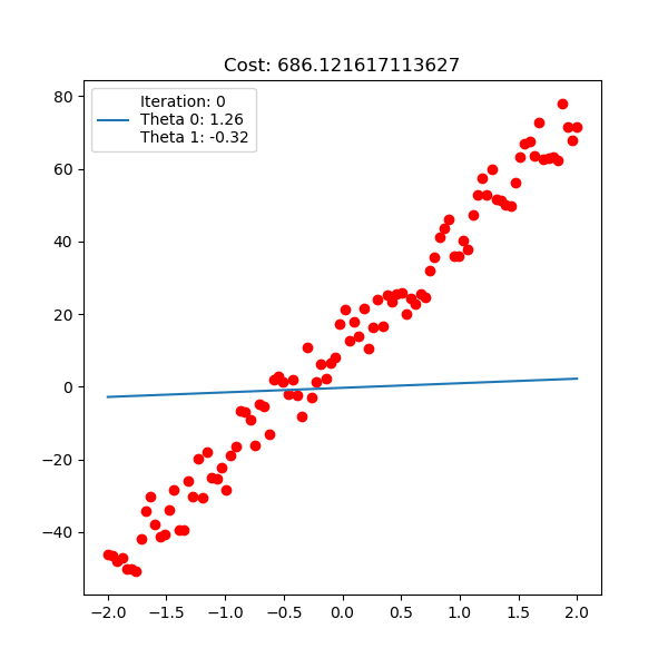
This is where gradient descent algorithm comes in. The idea of algorithm is at any point we move small step as backward direction of its derivative. The algorithm always make sure it will approach global minimum in finite steps with appropriate learning rate $\alpha$ (this is true for linear regression but not for other advanced models).
\[\mbox{Gradient descent: } \mathbf{w} = \mathbf{w} - \alpha \frac{\partial J(\mathbf{w}) }{\mathbf{w}} \mbox{ with } \alpha \mbox{ is the learning rate hyperparameter}\]If learning rate is too large, our update with derivative will blow up and it never converges. If learning is too small, the convergence is so slow, and probably no converge.
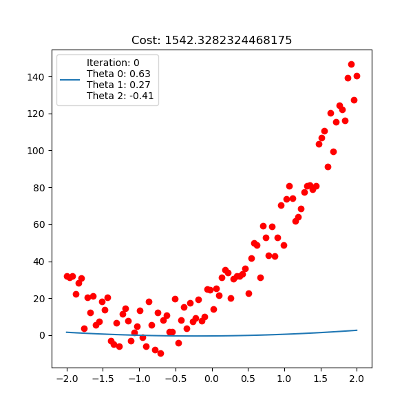
Below is polynomial linear regression, although it’s a curve but our optimization is still respect to $\mathbf{w}$ which is linear.
For linear regression implementation, checkout here.