Logistic Regression is a model using for classification problems. Although “regression” in its name but logistic regression uses mostly for classification problems, especially binary classification.
Logistic Regression uses sigmoid function as the output which is a popular activation function in neural network. It can understand as the conditional probability for true class given linear function.
\[\mbox{Dataset: }\mathbf{X} = (\mathbf{x_1}, \mathbf{x_2}, ..., \mathbf{x_n}) \in R^{N, D}\] \[\mbox{Linear function: } \mathbf{h} = \mathbf{X} \mathbf{w}\] \[\mbox{Logistic regression: }\mathbf{z} = \sigma(\mathbf{h}) = P(y = 1 | x) = \frac{1}{1 + e^{-\mathbf{h}}}\]The graph of sigmoid function:
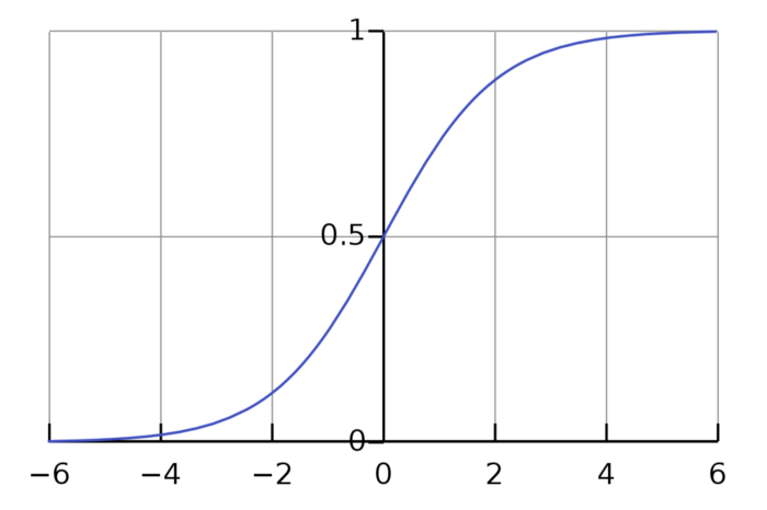
Graph of Sigmoid function.
We can see that its upper bound is 1 and lower bound is 0, this property makes sure we output a probability.
Intuitively, given a dataset with $\mathbf{X}$ is a matrix of features and $\mathbf{y}$ is vector label either positive or negative class, we want to classify which data point $\mathbf{x}_i$ belongs to. That means, visually, we find a line/plane/hyperplane (decision boundary) that split our data into 2 regions. That intuition is using mostly for SVM algorithm.
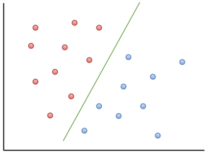
SVM: best line split data into 2 regions.
But, logistic regression intuition is different. It maps data points to a higher dimension, e.g: 2 dimension -> 3 dimension, with the new added dimension corresponding probability of classes. By default, I choose if data points have probability ≥ 0.5 is class 1, and class 0 otherwise.
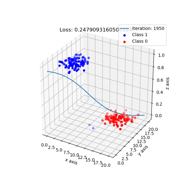
The shape of logistic regression mapping from 2D -> 3D.
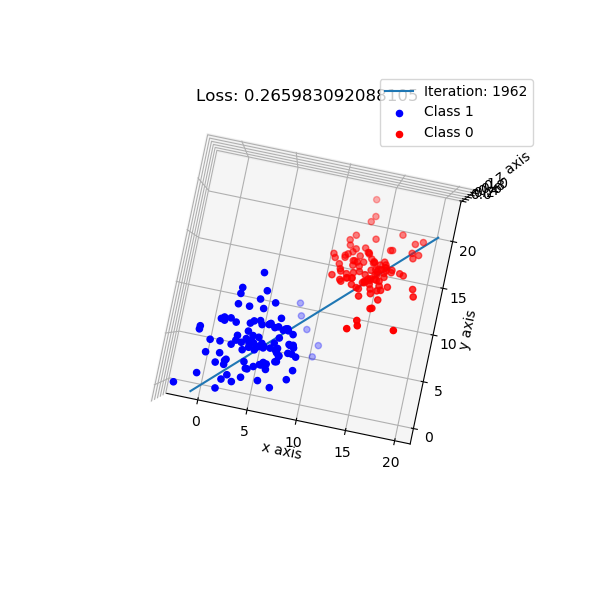
Look from top-down aspect.
Since sigmoid outputs probability, we use negative log likelihood to represent the error:
\[J = -\frac{1}{M}\sum_{i=1}^M(y_i log(z_i) + (1 - y_i)log(1 - z_i))\]where $M$ is number of data points, $y_i$ is true label, $z_i$ is predicted probability of sigmoid. We want to minimize this loss with respect to parameters $\mathbf{w}$.
\[\mbox{Use chain rule: } \frac{\partial J}{\partial \mathbf{w}} = \frac{\partial J}{\partial \mathbf{z}} \frac{\partial \mathbf{z}}{\partial \mathbf{h}} \frac{\partial \mathbf{h}}{\partial \mathbf{w}}\] \[\frac{\partial J}{\partial \mathbf{z}} = -\frac{1}{M}\left(\frac{\mathbf{y}}{\mathbf{z}} - \frac{1-\mathbf{y}}{1-\mathbf{z}}\right) = \frac{1}{M}\frac{\mathbf{z} - \mathbf{y}}{\mathbf{z}(1-\mathbf{z})}\] \[\frac{\partial \mathbf{z}}{\partial \mathbf{h}} = \mathbf{z}(1-\mathbf{z})\] \[\frac{\partial \mathbf{h}}{\partial \mathbf{w}} = \mathbf{X}\] \[\frac{\partial J}{\partial \mathbf{w}} = \frac{1}{M} \mathbf{X}^T (\mathbf{z}-\mathbf{y})\]Surprisingly, the derivative J with respect to $\mathbf{w}$ of logistic regression is identical with the derivative of linear regression. The only difference is that the output of linear regression is $\mathbf{h}$ which is linear function, and in logistic is $\mathbf{z}$ which is sigmoid function.
After found derivative we use gradient descent to update the parameters:
\[\mathbf{w} = \mathbf{w} - \alpha \frac{\partial J}{\partial \mathbf{w}}\]We’re sure that it will converge in finite steps.
For logistic regression implementation, checkout here.